
Control systems are everywhere — in your oven, car, air conditioner, and even in industrial robotics. To manage these systems efficiently, engineers use controllers that adjust the output to maintain a desired target value. One of the most common controllers is the Proportional-Integral (PI) Controller.
In this guide, we will cover everything about PI controllers — from the basics to step-by-step calculations, real-life applications, tuning methods, diagrams, and exam/IA strategies. By the end, students will have a complete understanding of this topic.
A PI controller is a type of feedback controller that uses two components:
Proportional (P): Reacts to the current error between the desired setpoint (SP) and the process variable (PV).
Integral (I): Reacts to the accumulated error over time, removing any residual error left by the proportional action.
Error formula:
Error = Setpoint (SP) − Process Variable (PV)
Key takeaway:
The P part reacts quickly to deviations.
The I part corrects any remaining differences over time.
Example:
Imagine you are heating water to 60°C. The P action increases the heater power immediately if the water is below 60°C. If the temperature remains slightly below 60°C due to constant heat loss, the integral action gradually increases heater power until the temperature reaches 60°C exactly.
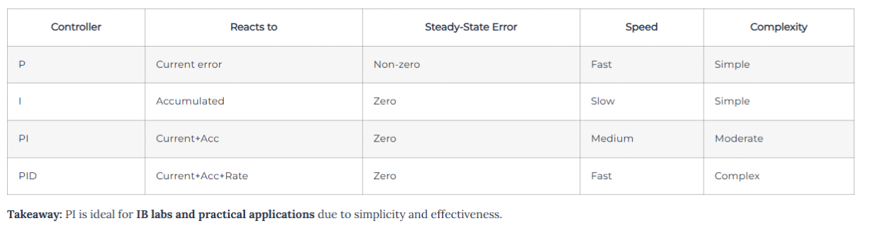
Using only P control can leave a steady-state error — the system never reaches the exact setpoint. Using only I control is too slow for practical use. The PI controller balances speed and accuracy:
Fast initial response: Proportional
Zero steady-state error: Integral
Practical Intuition
Consider driving at 60 km/h:
If your speed drops to 55 km/h, the proportional action increases acceleration immediately.
If you remain slightly below 60 km/h, the integral action gradually increases acceleration until exactly 60 km/h.
Thus, PI control gives smooth, accurate, and stable control.
The proportional component is calculated as:
P_output = Kp × error
Where Kp is the proportional gain.
How it works:
High Kp → system reacts strongly to errors; may overshoot
Low Kp → system reacts slowly; may never fully correct
Graphical representation:
Plot SP and PV vs. time
P-only response: quick rise but slight steady-state error remains
Error = 100 − 90 = 10

P_output = 2 × 10 = 20
The output of 20 units (volts, percentage, etc.) is applied to the system actuator.
The integral component addresses accumulated error over time:
I_output = Ki × ∫ error dt
Ki = integral gain
∫ error dt = cumulative error over time
Key points:
Eliminates steady-state error
Works slower than P
Too high Ki → overshoot; too low Ki → slow correction
Suppose error = 2°C over 10 seconds, Ki = 0.5
I_output = 0.5 × (2 × 10) = 10
This output slowly corrects the residual error.
Combined output formula:
Output = Kp × error + Ki × ∫ error dt
Workflow:
Measure PV
Calculate error (SP − PV)
Compute P_output
Compute I_output
Sum P + I → actuator
System responds → new PV
Repeat
Insight:
P reacts immediately
I removes residual errors
This dual-action approach is what makes PI control widely used.
Continuous-time formula:
u(t) = Kp × e(t) + Ki × ∫ e(t) dt
Where:
u(t) = controller output
e(t) = SP − PV
Kp = proportional gain
Ki = integral gain
Discrete-time formula (useful in IB IAs / simulations):
u[n] = Kp × e[n] + Ki × sum(e[0..n] × dt)
n = discrete time step
dt = time interval
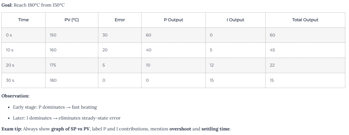
Goal: Maintain 2000 rpm under changing load
Load increases → RPM drops → error rises
P_output immediately increases voltage to motor
Small remaining error → I_output gradually eliminates it
Motor stabilizes at 2000 rpm
Graph suggestion: Plot SP, PV, P contribution, I contribution over time. This helps visualize how PI balances speed and accuracy.
Setpoint (SP): 100°C
PV: 90°C
Kp: 2
Ki: 0.5
Accumulated error: 10°C·s
Step 1: Error = SP − PV = 10
Step 2: P_output = Kp × error = 2 × 10 = 20
Step 3: I_output = Ki × accumulated_error = 0.5 × 10 = 5
Step 4: Total_output = 20 + 5 = 25
Interpretation: 25 units applied to the actuator will bring PV closer to SP.
Stepwise Method
Set Ki = 0
Increase Kp until fast response without oscillation
Slowly introduce Ki to remove steady-state error
Check for overshoot and stability
Adjust Kp and Ki iteratively
Consider anti-windup for actuator limits
Ziegler–Nichols Method (optional, advanced)
Increase Kp until sustained oscillation occurs (Ku)
Measure period of oscillation (Tu)
Set Kp = 0.45×Ku, Ki = 1.2×Kp/Tu
💡 For IB students: Stepwise tuning + plots + tables is sufficient.
Confusing I and D (integral vs derivative)
Not specifying units for Kp, Ki
Ignoring anti-windup
Using P alone → leaves steady-state error
Overestimating Ki → overshoot
✅ Always include graph, calculation, and explanation in IA or exam response.
Include block diagram of PI controller
Show step response graph
Label P and I contributions
Include numerical table of outputs
Discuss overshoot, settling time, and limitations
Mention real-world applications
💡 This demonstrates understanding, analysis, and evaluation — key for IA marks.
PI Block Diagram: Error → P → sum → Output; Error → I → sum → Output
Step Response Graph: SP vs PV over time
Contribution Graph: Show P and I contributions
Tuning Flowchart: Stepwise method
Tip: Use Excel, Google Sheets, or drawing software. Include labels and units.
Oven temperature control
HVAC systems
Motor speed and position
Robotics
Pressure and flow regulation
Medical devices (infusion pumps)
Takeaway: PI control is used anywhere precision regulation is needed.
Use Excel or Python for step-by-step simulations
Discrete-time formula:
u[n] = Kp * e[n] + Ki * sum(e[0..n]*dt)
Plot SP, PV, P, I contributions
IB IA tip: Include screenshots of simulation and describe trends.
Anti-windup techniques prevent integrator from overshooting
Sampling time (dt) affects discrete-time controller accuracy
Noise filtering can be necessary in derivative systems (PID)
Include keyword naturally in H1, first paragraph, subheadings, FAQ
Use people-first language — helpful content for students
Add diagrams with alt text
Include internal links: IB Math integration, Physics control systems, IA samples
Use FAQ schema for Google results
Ensure mobile-friendly, fast-loading page
Controller using current error + accumulated past error to reach and maintain setpoint.
PID adds derivative term to anticipate trends; PI is simpler.
When integral accumulates too much while actuator is saturated → overshoot. Prevent with anti-windup.
Temperature, motor control, robotics, pressure regulation, medical devices.
Stepwise method: tune Kp first, then Ki, monitor response, adjust iteratively.
Yes. Use discrete-time formula and plot SP, PV, P, I contributions.
IB Demystified is a trusted online learning platform led by certified IB examiners and educators.
© 2026 IB Demystified LTD ALL RIGHTS RESERVED. Powered by AfiaDigital
WhatsApp us